Page Not Found
Page not found. Your pixels are in another canvas.

A list of all the posts and pages found on the site. For you robots out there is an XML version available for digesting as well.
Page not found. Your pixels are in another canvas.
About me
This is a page not in th emain menu
Published:
This post will show up by default. To disable scheduling of future posts, edit config.yml and set future: false.
Published:
This is a sample blog post. Lorem ipsum I can’t remember the rest of lorem ipsum and don’t have an internet connection right now. Testing testing testing this blog post. Blog posts are cool.
Published:
This is a sample blog post. Lorem ipsum I can’t remember the rest of lorem ipsum and don’t have an internet connection right now. Testing testing testing this blog post. Blog posts are cool.
Published:
This is a sample blog post. Lorem ipsum I can’t remember the rest of lorem ipsum and don’t have an internet connection right now. Testing testing testing this blog post. Blog posts are cool.
Published:
This is a sample blog post. Lorem ipsum I can’t remember the rest of lorem ipsum and don’t have an internet connection right now. Testing testing testing this blog post. Blog posts are cool.
Published:
 The water in Zurish is very very clean.
Published:
 The beautiful summer vacation started from Berlin.
Published:
A very happy day
Published:
 The beautiful and peaceful night of Leiden.
Published in Journal, 2019
This paper is the work done in Hong Kong Baptist University.
Recommended citation: Wang, Y., Lan, W., Li, N., Lan, Z., Li, Z., Jia, J., & Zhu, F. (2019). Stability of Nonfullerene Organic Solar Cells: from Built‐in Potential and Interfacial Passivation Perspectives. Advanced Energy Materials, 9(19), 1900157. https://onlinelibrary.wiley.com/doi/full/10.1002/aenm.201900157
Published in Journal, 2019
A wideband circularly polarized (CP) dielectric resonator antenna (DRA) loaded with the partially reflective surface for gain enhancement is presented in this article. First, the DRA is excited by a microstrip line through modified stepped ring cross‐slot to generate the circular polarization. Four modified parasitic metallic plates are sequentially placed around the DRA for greatly widening the axial‐ratio bandwidth. Then, a partially reflective surface is introduced for enhancing the gain performance and further improving the CP bandwidth as well. Finally, an optimized prototype is fabricated to verify the design concept. The measured results show that the proposed DRA achieves 54.3% impedance bandwidth (VSWR<2) and 54.9% 3‐dB AR bandwidth. Besides, its average and peak gains are 10.7 dBic and 14.2 dBic, respectively. Wide CP band and high gains make the proposed DRA especially attractive for some broadband wireless applications such as satellite communication and remote sensing.
Recommended citation: Wen, J., Jiao, Y. C., Zhang, Y. X., & Jia, J. (2019). Wideband circularly polarized dielectric resonator antenna loaded with partially reflective surface. International Journal of RF and Microwave Computer‐Aided Engineering, 29(12), e21962. https://onlinelibrary.wiley.com/doi/full/10.1002/mmce.21962
Published in Conference, 2021
This paper is accepted by ISBI2021.
Recommended citation: Jia, J., Zhai, Z., Bakker, M. E., Hernández-Girón, I., Staring, M., & Stoel, B. C. (2021, April). Multi-task Semi-supervised Learning for Pulmonary Lobe Segmentation. In 2021 IEEE 18th International Symposium on Biomedical Imaging (ISBI) (pp. 1329-1332). IEEE. https://ieeexplore.ieee.org/abstract/document/9433985
Published in Conference, 2021
This paper is accepted by SPIE2022.
Recommended citation: Jingnan Jia, Marius Staring, Irene Hernández-Girón, Lucia J. M. Kroft, Anne A. Schouffoer, Berend C. Stoel. Prediction of Lung CT Scores of Systemic Sclerosis by Cascaded Regression Neural Networks. arXiv preprint arXiv:2110.08085. https://arxiv.org/ftp/arxiv/papers/2110/2110.08085.pdf
Published in Conference, 2021
This paper is published by IEEE Access.
Recommended citation: Jia, Jingnan, Emiel R. Marges, Jeska K. De Vries-Bouwstra, Maarten K. Ninaber, Lucia JM Kroft, Anne A. Schouffoer, Marius Staring, and Berend C. Stoel. "Automatic pulmonary function estimation from chest CT scans using deep regression neural networks: the relation between structure and function in systemic sclerosis." IEEE Access 11 (2023): 135272-135282. https://ieeexplore.ieee.org/stamp/stamp.jsp?arnumber=10330905
Published:
On Monday’s Lab Meeting, I gave a presentation on my current work: Multi-task Semi-supervised Deep Learning for lung lobe segmentation in CT.
Published:
This is a casual and brief introduction on Mandarin Chinese. The used material is here.
Published:
ISBI 2021 was hold online because of Covid-19. I gave the presentation of our accepted paper.
Published:
On Monday’s Lab Meeting, I gave a presentation on my work: Prediction of Lung CT Scores of Systemic Sclerosis by an End-to-end Fully Automatic Framework using Deep Learning.
Published:
A brief introduction on MONAI (a PyTorch-based framework for deep learning in healthcare imaging) and my experience on MONAI bootcamp 2021 (https://www.gpuhackathons.org/event/monai-miccai-bootcamp-2021). All materials are here.
Published:
SPIE 2022 was hold online because of Covid-19. I gave the presentation of our accepted paper.
Published:
python setup.py sdist bdist_wheel
twine upload dist/*
Published:
Record some knowledge I need to know for MeVisLab.
Published:
Published:
As the teaching assitant, I need to be familar with MATLAB more. The following commands will be used in courses.
Published:
Some jupyter notebook use tips.
Published:
Published:
This will record how to add google analytics. I can check the visitor count now from google analytics. The next step is to show it in the web.
Published:
Published:
Checklist for Remote cluster working
Published:
Itemss you need to know for your AI project.
Published:
The first time I touched MONAI is from a challenge: COVID-19 Lung CT Lesion Segmentation Challenge - 2020. The official originizer provided a banchmark implemented by MONAI.
Published:
MLflow is an open source platform to manage the ML lifecycle, including experimentation, reproducibility, deployment, and a central model registry.
Published:
As a technical blog, with the increasement of contents, it becomes difficult to remember all the things you have written down. Thast’s why we need a Search function for our website.
Published:
Record some tools and packages I used in case I need them in the future.
Published:
Once we built a project/package, we need to tell the users how to use it. Normally we could write a manual. But with the update of the code, the manual needs to be updated at the same time. How to synthesize the update of the manual? We need to use some automatic tools to automate the pipeline. This blog will tell you how to build your Documentation automatically.
Published:
略微了解一下前端知识,方便构建自己的网站。 
Published:
Record some Linux commands I used in case I need them in the future.
Published:
Comparision between Packaging commands in Ruby and Python.
Published:
This blog will show the step-by-step experience building my own academic website.
Published:
I checked a great number of blogs about how to build a dual-language website. Most of them need to write seperate content by myself for two languages which is not what I expected. So I finally found my own method to achieve it.
Published:
How to set path is a hot discussed topic.
Published:
PyCharm and VS Code provide remote debugging features. Let’s see how to implement it, respectively.
Before continue, you need to know some knowledge on ssh from my previous blog.
Placeholder
Before remote development, we need to config the SSH for VS Code.
remote development extension.remote explore, click SSH targetsconfig, add the following code to SSH configeration file XXX\.ssh\config Host remote1
HostName remote-host-name
User username
IdentityFile XXX\.ssh\id_rsa
IdentityFile path should be the private key path which was generated following this blog (If you have already generate the key in VS Code terminal, then you can remote this line)The above content can also be found as the first chapter of this blog.But the second part of this blog is too complex. Do not use it.
After we successfully connect to remote machine, we can open the remote directory/file using VS Code and run the code directly using the remote Python interpreter (ctrl+shift+p -> Python: interpreter to select your prefer interpreter).
The same process with the aforementioned No gateway method, the only thing we need to pay attention is to build password-less SSH connection via gateway following this blog
Host remote2
  HostName remote-host-name
  User username
  ProxyJump username@gateway-host-name:22
Published:
今天想使用VS Code的远程debug功能,所以需要回忆一下SSH的相关知识。
简单说,SSH是一种网络协议,用于计算机之间的加密登录。如果一个用户从本地计算机,使用SSH协议登录另一台远程计算机,我们就可以认为,这种登录是安全的,即使被中途截获,密码也不会泄露。最早的时候,互联网通信都是明文通信,一旦被截获,内容就暴露无疑。1995年,芬兰学者Tatu Ylonen设计了SSH协议,将登录信息全部加密,成为互联网安全的一个基本解决方案,迅速在全世界获得推广,目前已经成为Linux系统的标准配置。 SSH只是一种协议,存在多种实现,既有商业实现,也有开源实现。本文针对的实现是OpenSSH,它是自由软件,应用非常广泛。这里只讨论SSH在Linux Shell中的用法。如果要在Windows系统中使用SSH,会用到另一种软件PuTTY,这需要另文介绍。
SSH之所以能够保证安全,原因在于它采用了公钥加密。 整个过程是这样的:
这个过程本身是安全的,但是实施的时候存在一个风险:如果有人截获了登录请求,然后冒充远程主机,将伪造的公钥发给用户,那么用户很难辨别真伪。因为不像https协议,SSH协议的公钥是没有证书中心(CA)公证的,也就是说,都是自己签发的。 可以设想,如果攻击者插在用户与远程主机之间(比如在公共的wifi区域),用伪造的公钥,获取用户的登录密码。再用这个密码登录远程主机,那么SSH的安全机制就荡然无存了。这种风险就是著名的”中间人攻击”(Man-in-the-middle attack)。
SSH主要用于远程登录服务器(主要是Linux服务器),进行代码部署、运行、debugging等。
Linux系统上有开源软件openssh可以实现ssh协议。OpenSSH分客户端openssh-client和服务器端openssh-server
如果你只是想登陆别的机器的SSH只需要安装openssh-client(ubuntu有默认安装,如果没有则sudoapt-get install openssh-client),如果要使本机开放SSH服务就需要安装openssh-server。
运行在服务器上的Linux系统默认已经安装了SSH-server. 运行在用户端的Ubuntu等很多Linux系统默认已经安装了ssh client。 尽管如此,如果你想给一个Linux系统安装ssh的服务器端或/和客户端,请看此文。
Windows一般极少作为服务器端,不过如果你发现一台Windows服务器,它大概率都是拥有ssh服务器端功能的。运行在用户端的Windows系统不一定有SSH客户端,需要安装SSH客户端软件。如何安装请看下文。
Windows和linux都有很多专门的SSH客户端软件(或者具有SSH客户端功能的软件)。只是Windows系统的客户端软件一般有UI界面,Linux系统的客户端软件一般没有UI界面,通过命令行运行。
更多见此博文。
从上文的SSH原理可知,SSH 默认采用密码登录,这种方法有很多缺点,简单的密码不安全,复杂的密码不容易记忆,每次手动输入也很麻烦。所以,密钥登录是更好的解决方案。秘钥登录又称为免密(码)登录。
使用密码登录时候,客户端不需要生成或者使用自己的私钥或公钥,整个过程使用服务器端的公钥即可。但是客户端使用秘钥登录的话,需要自己生成自己的私钥公钥对,然后把公钥传给服务器端。具体登录的原理如下:
利用密钥生成器制作一对密钥——一只公钥和一只私钥。将公钥添加到服务器的某个账户上,然后在客户端利用私钥即可完成认证并登录。这样一来,没有私钥,任何人都无法通过 SSH 暴力破解你的密码来远程登录到系统。此外,如果将公钥复制到其他账户甚至主机,利用私钥也可以登录。
具体登录过程如下: SSH 密钥登录分为以下的步骤。
预备步骤,客户端通过ssh-keygen生成自己的公钥和私钥。
具体执行命令详见网上其他文章。
比如用MobaXterm去免密码连接多个服务器,需要在MobaXterm里生成多个秘钥对吗? 答案是:不需要。通常,我们只会生成一个SSH Key,名字叫id_rsa,然后提交到多个不同的网站(如:GitHub、DevCloud或Gitee)。再比如,我们在PowerShell上生成了一堆秘钥对之后把公钥传给多个服务器,就可以在PowerShell上免密码登录多个服务器。
一个客户端机器(Windows系统或者Linux系统)可以有很多SSH客户端软件。比如Windows上有PowerShell和MobaXterm。每个软件都可以生成SSH秘钥对,存放在各自软件对应的文件夹下(也可以自定义文件夹)。所以一个客户端机器是可能存在多个私钥公钥对的。
比如MobaXterm软件生成的秘钥对存放在C:\Users\jjia\DOCUME~1\MOBAXT~1\home\.ssh(可以通过在MobaXterm界面运行open /home/mobaxterm来弹出ssh所在文件夹)。通过MobaXterm运行ssh命令默认都会调用这里的秘钥对。
所以在MobaXterm里配置过后,可以通过MobaXterm免密登录。但是不代表这个配置可以同步应用到其他软件(比如PowerShell或者VS Code)。因为其他软件可能应用的是不同文件夹下的不同的私钥,因此对于其他软件又需要按照类似的方法单独配置免密登录。比如,我在MobaXterm里生成了秘钥对,把MobaXterm默认的.ssh文件夹下的公钥复制到remote server上。但是VS Code是没法使用的。我需要在VS Code的终端重新生成秘钥对,然后重新把新的秘钥对添加到远程的服务器上。注意不要覆盖掉远程服务器之前的公钥。具体可以采用ssh-copy-id -i ~/.ssh/id_rsa.pub <user-name>@server.xxx.xxx的方式。对于有gateway的情况,需要先复制公钥到gateway: ssh-copy-id -i ~/.ssh/id_rsa.pub <user-name>@gateway.xxx.xxx,再复制公钥到remote server: ssh-copy-id -i ~/.ssh/id_rsa.pub <user-name>@server.xxx.xxx。
或者,在其他软件中专门设置去调用MobaXterm里生成的秘钥对 (但是我对如何设置并没有太多经验,这里留待其他人补充)。
存在另一种需要,我们在同一个网站上,注册了两个用户名,通常网站不会允许我们为这两个用户名,配置同一个SSH Key,这时候就会有些麻烦。我们就需要在一台电脑上,如何配置多个SSH Key.
详见此文
Take my ssh config as an example.
Host login2tunnel
    HostName xxx.xxx.xxx
    User myname
    ProxyJump [email protected]:22
    LocalForward 5000 localhost:5000
    LocalForward 22 xxx.xxx.xxx:22
    ServerAliveInterval 60
参考资料:
Published:
我们首先要了解域名和IP地址的区别。IP地址是互联网上计算机唯一的逻辑地址,通过IP地址实现不同计算机之间的相互通信,每台联网计算机都需要通过IP地址来互相联系和分别。
但由于IP地址是由一串容易混淆的数字串构成,人们很难记忆所有计算机的IP地址,这样对于我们日常工作生活访问不同网站是很困难的。基于这种背景,人们在IP地址的基础上又发展出了一种更易识别的符号化标识,这种标识由人们自行选择的字母和数字构成,相比IP地址更易被识别和记忆,逐渐代替IP地址成为互联网用户进行访问互联的主要入口。这种符号化标识就是域名。
域名虽然更易被用户所接受和使用,但计算机只能识别纯数字构成的IP地址,不能直接读取域名。因此要想达到访问效果,就需要将域名翻译成IP地址。而DNS域名解析承担的就是这种翻译效果。
对于托管在github上的我们的个人网站,如果我们想给它新的域名,我们需要把新的域名映射到github的服务器上去。
域名解析详细过程参见原文章
我个人主要学习了原文章中的以下知识:
主要分为A记录、MX记录、CNAME记录、NS记录和TXT记录:
1、A记录
A代表Address,用来指定域名对应的IP地址,如将item.taobao.com指定到115.238.23.xxx,将switch.taobao.com指定到121.14.24.xxx。A记录可以将多个域名解析到一个IP地址,但是不能将一个域名解析到多个IP地址
2、MX记录
Mail Exchange,就是可以将某个域名下的邮件服务器指向自己的Mail Server,如taobao.com域名的A记录IP地址是115.238.25.xxx,如果将MX记录设置为115.238.25.xxx,即[email protected]的邮件路由,DNS会将邮件发送到115.238.25.xxx所在的服务器,而正常通过Web请求的话仍然解析到A记录的IP地址
3、CNAME记录
Canonical Name,即别名解析。所谓别名解析就是可以为一个域名设置一个或者多个别名,如将aaa.com解析到bbb.net、将ccc.com也解析到bbb.net,其中bbb.net分别是aaa.com和ccc.com的别名
4、NS记录
为某个域名指定DNS解析服务器,也就是这个域名由指定的IP地址的DNS服务器取解析
5、TXT记录
为某个主机名或域名设置说明,如可以为ddd.net设置TXT记录为”这是XXX的博客”这样的说明
所以我将我买了域名之后,设置如下: 
购买域名以及如何设置新域名,我另一篇文章有描述。
Published:
You may think that yourname.github.io is not cool enough compared with yourname.com. No worries, we can change the domain.
NOte: the following steps could also be found on official documentation
https instead of http. Some browsers will alear unsafe if your website starts with http.username.github.io, click Code and automation-> Pages -> Custom domain -> enter www.yourname.com -> Save.Dashboard -> manage -> Advanced DNS, set DNS like the following figure. The IP address in the following screenshot is the IP address of github servers. You can also copy them from the official documentation Then you need to wait for several hours to 24 hours. You can check the DNS status on setting of your repository. It looks like the followinig figures. If it shows unsuccessful, you can try again.

Set SSL.
SSL can change your domain from http to https, so that browser would think your website become Safe. Otherwise, your website would look like: 
So how to set SSL? `At first you need to buy it from your domain provider. After that you need to install and activate it.` DO NOT BUY SSL! Because Github itself provides very simple method to achieve it. Just go to the setting of your repository username.github.io, click Code and automation-> Pages -> Check Enforce HTTPS. You may need to wait for several minutes to observe its influence, and you may see the layout of the whole website broke down during these minites. You can try another browser, or clear the browser cache (e.g. Chrome incognito) and try to visit the website again. Please be patient and you will see the perfect performance finally.
Published:
The minimal important difference (MID) or minimal clinically important difference (MCID) is the smallest change in a treatment outcome that an individual patient would identify as important and which would indicate a change in the patient’s management.
Published:
在学习MCID(最小临床差异)的时候,量表这个概念多次被提到。所以这里谈一谈量表。
Published:

From the above image (several voxels in 3D image) we can observe that in 3D image, two neighboring pixels could have 3 different relationships: face-connected (red voxel VS gray voxel, distance=1), edge-connected (red voxel VS blue voxel, distance=sqrt(2)) and corner-connected (red voxel VS green voxel, distance=sqrt(3)).
Therefore, given red voxel is the object, drawing its border could have 3 different results: face-connected (only gray voxel is the border, distance=1), edge-connected (gray and blue voxels are the border, where the distance is equal to or less than sqrt(2)) and corner-connected (gray, blue and green voxels are all the border, where the distance is equal to or less than sqrt(3)).
2D image only has face-connected neighbors and edge-connected neighbors.
Note: This post is to illustrate the fully_connected argumennt in seg-metrics
Published:
CNN通常由一些卷积块(卷积层+激活层+池化层)和全连接层组成。 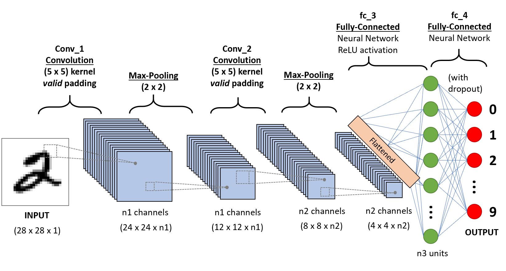
CNN的可解释性可以通过以下几种方式进行。
通过直接展示中间层的特征图(一般要归一化到0-256之间),观察经过每一层卷积之后图片的变化。如下图。  上图为某CNN 5-8 层输出的某喵星人的特征图的可视化结果(一个卷积核对应一个小图片)。可以发现越是低的层,捕捉的底层次像素信息越多,特征图中猫的轮廓也越清晰。越到高层,图像越抽象,稀疏程度也越高。这符合我们一直强调的特征提取概念。
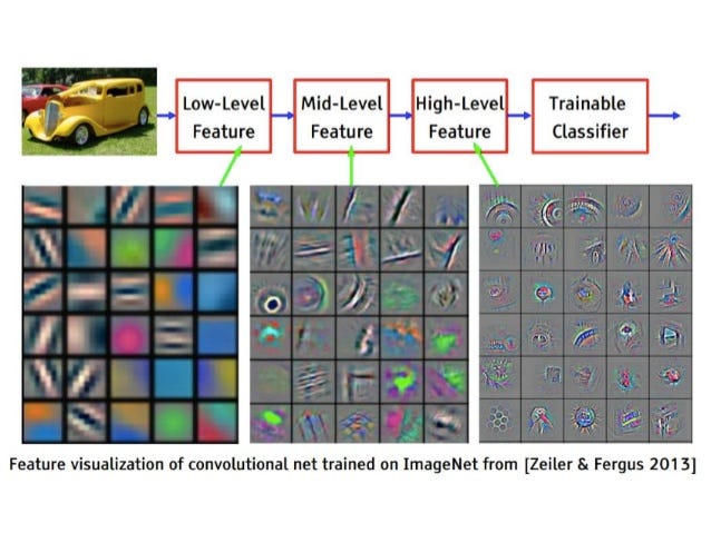
想要观察卷积神经网络学到的过滤器,一种简单的方法是获取每个过滤器所响应的视觉模式。我们可以将其视为一个优化问题,即从空白输入图像开始,将梯度上升应用于卷积神经网络的输入图像,让某个过滤器的响应最大化,最后得到的图像是选定过滤器具有较大响应的图像。  更多图片和解释见此文
从而得到下面2张图。图中前几层看起来是纹理,后几层是更高级的综合性的信息

问题1: 为什么上面2张图中后面的特征图反而像素更高?难道不是后面的特征图的尺寸更小,像素更低吗? 答案1: 因为这并不是直接的特征图可视化,而是DeConv: 把中间层的特征,一层一层反传到输入端口,使得特征图的尺寸逐步放大到和输入图片相同 (原文:”map these activities back to the input pixel space, showing what input pattern originally caused a given activation in the feature maps”)。
问题2 这个DeConvnet生成的图,输入是什么?是最后一个卷积块的输出(全连接层之前)? 答案2 论文原话:”To examine a given convnet activation, we set all other activations in the layer to zero and pass the feature maps as input to the attached deconvnet layer”.
问题2:backpropagation, deconvnet 和guided backgpropagati的区别是什么? **答案2 导向反向传播与反卷积网络的区别在于对ReLU的处理方式。在反卷积网络中使用ReLU处理梯度,只回传梯度大于0的位置,而在普通反向传播中只回传feature map中大于0的位置,在导向反向传播中结合这两者,只回传输入和梯度都大于0的位置,这相当于在普通反向传播的基础上增加了来自更高层的额外的指导信号,这阻止了负梯度的反传流动,梯度小于0的神经元降低了正对应更高层单元中我们想要可视化的区域的激活值(https://blog.csdn.net/KANG157/article/details/113154590) 
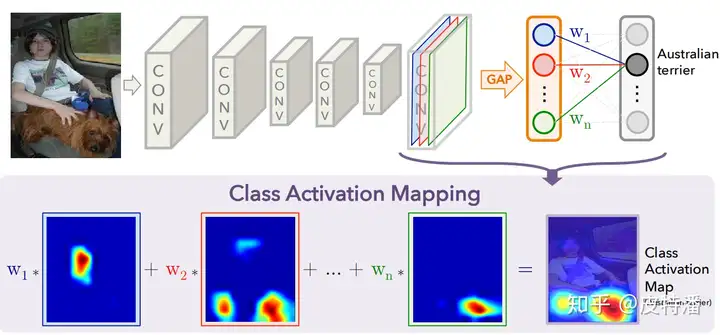
CAM是一系列类似的激活图。大致原理是把最后一层卷积所输出的特征图通过加权和组成一张图。权重的设计不同产生了一系列不同的论文。  下面一个一个介绍。
该方法的缺点是只能适用于最后一层特征图和全连接之间是GAP操作。 如果不是,就需要用户修改网络并重新训练(或 fine-tune)。所以对本文简单概括即为:修改网络全连接为GAP形式,利用GAP层与全连接的权重作为特征融合权重,对特征图进行线性融合获取CAM。
对获取的特征图进行channel-wise遍历,对每层特征图进行上采样+归一化,与原始图片进行pixel-wise相乘融合,然后送进网络获取目标类别score(softmax后),减去baseline(全黑图片)的目标类别score,获取CIC。再进行softmax操作来保证所有CIC之和为1。最后将CIC作为特征融合权重融合需要可视化的特征层。
If we change one pixel in our input image, how much will it affect the final probability score?
Well, first of all, one way to calculate this is to perform a backpropagation and to calculate a gradient of the score with respect to this pixel value. This is easily doable in PyTorch. Then, we can repeat this process for all pixels and record the gradient values. As a result, we will get high values for the location of a dog. Note, that in this example we get a “ghostly image” of a dog, signifying that the network is looking in the right direction!
参考文献:
Published:
Reference:
Published:
Answer:
I do not believe it. Or I think PFT regression net should be sensitive to smalll (organ) perturbation. Pooling will lose such information. I want to try if No-Pooling can lead to the same performance.
Published:
假设检验(hypothesis testing),又称统计假设检验,是用来判断样本与样本、样本与总体的差异是由抽样误差引起还是本质差别造成的统计推断方法。显著性检验是假设检验中最常用的一种方法,也是一种最基本的统计推断形式,其基本原理是先对总体的特征做出某种假设,然后通过抽样研究的统计推理,对此假设应该被拒绝还是接受做出推断。常用的假设检验方法有Z检验、t检验、卡方检验、F检验等。
假设检验的基本思想是“小概率事件”原理,其统计推断方法是带有某种概率性质的反证法。小概率思想是指小概率事件在一次试验中基本上不会发生。反证法思想是先提出检验假设,再用适当的统计方法,利用小概率原理,确定假设是否成立。即为了检验一个假设H0是否正确,首先假定该假设H0正确,然后根据样本对假设H0做出接受或拒绝的决策。如果样本观察值导致了“小概率事件”发生,就应拒绝假设H0,否则应接受假设H0。
个人笔记:比如我假设A方法和B方法效果相同(这是针对总体特征的假设),为了检验这个假设是否正确,首先假定该假设H0正确。然后根据样本(A方法产生a组数据100个,均值为3.4,B方法产生b组数据100个,均值为3.6)对假设H0做出接受或拒绝的决策。如果样本观察值导致了“小概率事件”发生(计算a组的SD和b组的SD,结合),就应拒绝假设H0,否则应接受假设H0。
Published:
Published:
绝大部分的Python包可以通过pip install [package_name]来安装。因为绝大部分Python包都会被上传到PyPi.
对于conda的用户,另一种常用的方式是conda install [package_name]。但是其实并不是所有的包都会被上传到conda所维护的服务器上。对于Python包的开发者而言,第一选择肯定是传到Python官方的包托管平台PyPi上,如果还有时间或者想进一步推广自己的包的话,会选择再把自己的包上传到conda的包托管平台。而且conda有两个包托管的源:Anaconda公司自己维护的源(包质量比较稳定,更新较慢)和社区维护的conda-forge(更新较快)。
一般我们自己写好了Python包之后,如果只给自己用,一般可以通过两种方式:
from .. import [module_name] import sys
sys.path.append(r'E:\src\ttlayer')
sys.path.insert(0,r'E:\src\ttlayer')
在Linux里导入
方法1:
export PATH=/home/uusama/mysql/bin:$PATH
# 或者把PATH放在前面
export PATH=$PATH:/home/uusama/mysql/bin
注意事项: 生效时间:立即生效 生效期限:当前终端有效,窗口关闭后无效 生效范围:仅对当前用户有效 配置的环境变量中不要忘了加上原来的配置,即$PATH部分,避免覆盖原来配置
方法2: 通过修改用户目录下的~/.bashrc文件进行配置.在最后一行加上: export PATH=$PATH:/home/uusama/mysql/bin 注意事项: 生效时间:使用相同的用户打开新的终端时生效,或者手动source ~/.bashrc生效 生效期限:永久有效 生效范围:仅对当前用户有效 如果有后续的环境变量加载文件覆盖了PATH定义,则可能不生效
What is the difference between the above 4 commands? Answer: This link
Published:
Published:
At first, I tried to install it on cluster, but enven it successfully installed, it raised ERROR during importing it in Python. This is because it require glibc higher than 2.18 or 2.27 (newest version). But my cluster has glibc of version 2.17.
Then, I tried to install it on my own workstation but still faied because my own workstation does not have a good GPU I think.
Finally, I installed it on my own PC using “pip install open3d” in a brand new conda environment.
torch.Tensor using Tensor Published:
torch.Tensor using Tensor?In numpy.Aarray or torch.Tensor, we have the following methods to index an Array or Tensor:
np_a = np.random.randn((30,4,5))
ts_a = torch.randn((30,4,5))
int number to index one elementtmp = np_a[1]
tmp = ts_a[1]
start:end to index a range of continuous elementstmp = np_a[10:13]
tmp = ts_a[:13]
tmp = np_a[:-2]
e.g. select the 1st, 3rd, 8th, and 29th element from np_a.
e.g. select the [0,0,0] and [1,1,1] and [20,1,2] three elements. #
a = np.arange(12)**2  # the first 12 square numbers
i = np.array([1,1,3,8,5])
a[i]  # array([ 1,  1,  9, 64, 25])

j = np.array([[3, 4], [9, 7]])  # a bidimensional array of indices
a[j]  # the same shape as `j` array([[ 9, 16], [81, 49]])
https://numpy.org/doc/stable/user/quickstart.html#advanced-indexing-and-index-tricks
Answer: The ‘multiple Arrays’ should have the same shapes and the number of Arrays should be the same as the dimensions of the target Array_T. Then the output Array has the same shape with the indexing Arrays.
e.g.
Arr_T = np.ones((5,6))
Arr_idx = np.ones((2,3,4))
Arr_T[Arr_idx,Arr_idx]
It does not matter. The output Array has the same shape with Arr_idx.
Note: The first and second method also apply to list.
Published:
Today I learnt how to use MLFlow in Databricks [1].
By the way, today I just found that MLFlow is released and maintained by Databricks! Databricks is so great!
This tutorial covers the following steps:
References:
In python [2]:
# restore experiments
from mlflow import MlflowClient

def print_experiment_info(experiment):
    print("Name: {}".format(experiment.name))
    print("Experiment Id: {}".format(experiment.experiment_id))
    print("Lifecycle_stage: {}".format(experiment.lifecycle_stage))

# Create and delete an experiment
client = MlflowClient()
experiment_id = client.create_experiment("New Experiment")
client.delete_experiment(experiment_id)

# Examine the deleted experiment details.
experiment = client.get_experiment(experiment_id)
print_experiment_info(experiment)
print("--")

# Restore the experiment and fetch its info
client.restore_experiment(experiment_id)
experiment = client.get_experiment(experiment_id)
print_experiment_info(experiment)
In python [2]:
from mlflow import MlflowClient

# Create a run under the default experiment (whose id is '0').
client = MlflowClient()
experiment_id = "0"
run = client.create_run(experiment_id)
run_id = run.info.run_id
print("run_id: {}; lifecycle_stage: {}".format(run_id, run.info.lifecycle_stage))
client.delete_run(run_id)
del_run = client.get_run(run_id)
print("run_id: {}; lifecycle_stage: {}".format(run_id, del_run.info.lifecycle_stage))
client.restore_run(run_id)
rest_run = client.get_run(run_id)
print("run_id: {}; lifecycle_stage: {}".format(run_id, res_run.info.lifecycle_stage))
In CLI [1]:
mlflow experiments delete [OPTIONS]
mlflow experiments restore [OPTIONS]
mlflow experiments search [OPTIONS]

mlflow gc [OPTIONS]  # delete the experiments permanently
In CLI [1]:
mlflow runs delete [OPTIONS]
mlflow runs restore [OPTIONS]  # --run-id <run_id>
mlflow runs list [OPTIONS]

mlflow gc [OPTIONS]  # delete the experiments permanently
References:
Published:
存储和数据直连,拓展性、灵活性差。 为了扩展,将文件和服务分离,通过网络连接——
设备类型丰富,通过网络互连,具有一定的拓展性,但是受到控制器能力限制,拓展能力有限。同时,设备到了生命周期要进行更换,数据迁移需要耗费大量的时间和精力。
通过网络使用企业中的每台机器上的磁盘空间,并将这些分散的存储资源构成一个虚拟的存储设备,数据分散的存储在企业的各个角落。
目前主流的分布式文件系统有:GFS、HDFS、Ceph、Lustre、MogileFS、MooseFS、FastDFS、TFS、GridFS等。
Reference:
Published:
A picture is worth a thousand words.

Summary: different models/folds have different prediction style (slope and intercept). If they are mised, the total r would be lower.
Comparing intraclass correlation to Pearson correlation coefficient (with R)
Published:

There are several metrics:
nvidia-smi)Here we only talk about FLOPs and parameters. Note: Floating point of operations (FLOPs) is different with floating point of per second (FLOPS). The FLOPS is the same for the same hardware device, but the FLOPs are different for different networks.
FLOPs is related to network design: Number of layers, activation layer selection, parameters, etc.
The difference between FLOPs and parameters is shown at the top figure.
Because Convolution layer can share the kernel, its parameters is far lower than the FLOPs.
PS: Throughput refers to the number of examples (or tokens) that are processed within a specific period of time, e.g., “examples (or tokens) per second”.
PS: Normally MACs (multiply–accumulate operation) are the half of FLOPs.
Published:
Normally I used a fixed random seed to split dataset. However, I found that my dataset has been slightly and gradually updated with the development of the project.
For instance, in the latter experiments, I found that some patients should be excluded. Then should I re-train all the previous expreiments again? if not, how to ensure the following experiments use the same training/validation/testing data with the previous experiment? (The same seed for different lenth of patient list will lead to very different data split)
So let’s use a YAML file to split dataset so that we can always have the almost same split for training/validation/testing data.
A complete YAML tutorial could be found at Real Python
Difference between YAML, JSON and XML is here
Published:
git push origin master
git remote set-url origin new.git.url/here
git remote show origin
How to let git remember my username and password?
$ git config credential.helper store
$ git push https://github.com/owner/repo.git

Username for 'https://github.com': <USERNAME>
Password for 'https://[email protected]': <PASSWORD>
可能是自己的用户名和邮箱号不对,Error提示一般如下:
$ git push origin master
remote: Permission to Jingnan-Jia/segmentation_metrics.git denied to jingnan222.
fatal: unable to access 'https://github.com/Jingnan-Jia/segmentation_metrics.git/': The requested URL returned error: 403
这个问题通常由以下原因造成: 因为你在用Windows!!!把仓库放到linux上就没有这些问题了!!!
如果您在本地创建了标签,但是在GitHub的远程仓库中不显示,很可能是因为标签没有被推送到远程仓库。Git的标签是不会自动随着git push命令推送的,除非您特别指定。
为了将标签推送到远程仓库,您需要执行以下命令:
推送单个标签:
git push origin <tagname>
将
推送所有标签:
git push origin --tags
这会将所有本地的标签推送到远程仓库。
请确保您执行了上述命令之一来推送标签。完成后,您应该能够在GitHub仓库的“Tags”部分看到您的新标签。
Published:
Some of my friends in mainland of China complained that they could not visit my website fluently. I need to do something to solve it!
Actually, I have tried to use Gitee or Coding (Chinese GitHub) to backup my current website and use soome technique to forward the visits to Gitee/Coding or GitHub according to the visitors’ location. However, Gitee and Coding is not free and they are not stable. The worse thing is that I have to push my code to Gitee/Coding and GitHub for each update of my website.
So I decided to accelerate my website using Cloudflare. It is free and stable.
Now lets see the steps.

Go to your domain’s provider website (mine is ‘namespace’), add the nameservers proveded by ‘cloudflare’ to it. 
References:
Published:
The shapes of different data are not the same, so they cannot be alligned or collated correctly.
The shape of the input and target for the loss function is very annoying. So I summarize them here.
predictions = torch.rand(2, 3, 4)
target = torch.rand(2, 3)
print(predictions.shape)
print(target.shape)
nn.CrossEntropyLoss(predictions.transpose(1, 2), target)  # the shape should be transposed!
RuntimeError: Expected object of scalar type Long but got scalar type Float for argument #2 'target'
input can be in any format, just targets should be in long.
# Example of target with class indices
loss = nn.CrossEntropyLoss()
input = torch.randn(3, 5, requires_grad=True)
target = torch.empty(3, dtype=torch.long).random_(5)  # target should be long
output = loss(input, target)
output.backward()

# Example of target with class probabilities
input = torch.randn(3, 5, requires_grad=True)
target = torch.randn(3, 5).softmax(dim=1)  # target with probabilities should be converted to between [0,1].
output = loss(input, target)
output.backward()
Because I used the monai.DiceLoss, the shape should be
Answer: change x to torch.tensor(x)
From the above link, it is observed that the most pupular datasets for point cloud classification is MOdelNet40 and ScanObjectNN.
For MOdelNet40 (released in 2015), in the top 10 networks, I first exclude the networks with extra training dataset, I can obtain:
They are all published in 2021 or 2022.
For ScanObjectNN (released in 2019), I first exclude the networks with extra training dataset, I can obtain:
They are all published in 2022.
Why the top networks for two datasets are so different? Which network should I choose for my dataset (PFT regression from binary vessel tree)?
ModelNet40 is synthetic, while ScanObjectNN is real-world dataset.
So I prefer to try the top networks in ScanObjectNN, which includes:
PointNet. Processed raw point sets through Multi-Layer Perceptrons (MLPs). While aggregating features at the global level using max-pooling operation, lost valuable local geometric information.
PointNet++. employed ball querying and k-Nearest Neighbor (k-NN) querying to query local neighborhoods to extract local semantic information. But it still lost contextual information due to the max-pooling operation
Published:
I want to get the fiel creation or docification time with seconds!!!
In windows, it seems impossible to see the exect time in Windows explorer, because it only shows the date and hour and minutes, missing the seconds!
Luckily, we have Python!
modified = os.path.getmtime(file)
print("Date modified: "+time.ctime(modified))
print("Date modified:",datetime.datetime.fromtimestamp(modified))

# out:
# Date modified: Tue Apr 21 11:50:46 2015
# Date modified: 2015-04-21 11:50:46
files.sort(key=os.path.getctime) from here.
Published:
https://www.tjelvarolsson.com/blog/five-exercises-to-master-the-python-debugger/
Published:
Timed out waiting for debuggee to spawnThis issue is pretty annoying! I coundnot find the solution.
Published:
How to balance the LaTex and Word?
Answer: Sending Word to supervisors if they preferred (convert LaTex to Word with pandoc if we already have LaTex version). Go back to LaTex in the final version.
From: https://www.zhihu.com/question/22316670
How to convert LaTex to Word? Answer1 (easiest and most correct way to convert PF to Word): use adobe online: https://www.adobe.com/acrobat/online/pdf-to-word.html Answer2: pandoc
Example:
 # in windows terminal
 pandoc main.tex -o main.docx
We need at first download pandoc.exe from https://pandoc.org/installing.html and save the pandoc.exe to the same directory with LaTex files.
Advanced Example;
pandoc input.tex --filter pandoc-crossref --citeproc --csl springer-basic-note.csl --bibliography=reference.bib -M reference-section-title=Reference -M autoEqnLabels -M tableEqns -t docx+native_numbering --number-sections -o output.docx
In the above example, the springer-basic-note.csl should be downloaded from https://www.zotero.org/styles?format=numeric and save it to the same directory with pandoc.exe. we can also download other styles like ieee from there.
The above advanced example requires pandoc-crossref which could be installed from: https://github.com/lierdakil/pandoc-crossref/releases
From:
1. https://blog.csdn.net/weixin_39504048/article/details/80999030
2. [Markdown 与 Pandoc](https://sspai.com/post/64842)
3. [使用 Pandoc 将 Latex 转化为 Word (进阶版本,包括引用图标和references) ](https://xhan97.github.io/latex/PandocLatex2Word.html)
How to cleaning up a .bib file?
Answer: manually clean it and check it.
Workflow: Write papers on overflow, download the source files, convert them to docx, send the docx to supervisors to review it, get the feedback, update the overflow (or just update the overflow in the final step before submission).
Published:
wandb login --relogin[0m to force relogin Thread HandlerThread: Traceback (most recent call last): File “/home/jjia/.conda/envs/py38/lib/python3.8/site-packages/wandb/sdk/internal/internal_util.py”, line 49, in run self._run() File “/home/jjia/.conda/envs/py38/lib/python3.8/site-packages/wandb/sdk/internal/internal_util.py”, line 100, in _run self._process(record) File “/home/jjia/.conda/envs/py38/lib/python3.8/site-packages/wandb/sdk/internal/internal.py”, line 280, in _process self._hm.handle(record) File “/home/jjia/.conda/envs/py38/lib/python3.8/site-packages/wandb/sdk/internal/handler.py”, line 136, in handle handler(record) File “/home/jjia/.conda/envs/py38/lib/python3.8/site-packages/wandb/sdk/internal/handler.py”, line 146, in handle_request handler(record) File “/home/jjia/.conda/envs/py38/lib/python3.8/site-packages/wandb/sdk/internal/handler.py”, line 697, in handle_request_run_start self._tb_watcher = tb_watcher.TBWatcher( File “/home/jjia/.conda/envs/py38/lib/python3.8/site-packages/wandb/sdk/internal/tb_watcher.py”, line 120, in init wandb.tensorboard.reset_state() File “/home/jjia/.conda/envs/py38/lib/python3.8/site-packages/wandb/sdk/lib/lazyloader.py”, line 60, in getattr module = self._load() File “/home/jjia/.conda/envs/py38/lib/python3.8/site-packages/wandb/sdk/lib/lazyloader.py”, line 35, in _load module = importlib.import_module(self.name) File “/home/jjia/.conda/envs/py38/lib/python3.8/importlib/init.py”, line 127, in import_module return _bootstrap._gcd_import(name[level:], package, level) File “More information: https://developers.google.com/protocol-buffers/docs/news/2022-05-06#python-updates wandb: ERROR Internal wandb error: file data was not synced
```
I havenot found the reason.
Published:
环境变量是指当在终端运行命令的时候,从哪些文件夹去找这个命令。比如python有很多个也许,用哪一个文件夹里的python呢?就需要沿着环境变量里的所有文件夹一个一个去找,一旦找到就停止,不再继续。
echo $PATH # in one lineecho -e ${PATH//:/\\n} # line by lineimport sys
sys.path.append("/home/my/path)
echo $PATH可以验证。这时候需要搞清楚$PATH怎么就被改动了?去看看.bashrc,那里面可能会发现export PATH=”your/new/path:$PATH”,大概率就是对$PATH进行改动的代码(新路径插入到开头去了)。注释掉或者调整路径添加的顺序就好了。Reference:
Published:
ModelNet ModelNet是帶顏色的! (reference: https://blog.csdn.net/weixin_47142735/article/details/120223827)
.off那个是CAD模型,modelnet40_ply_hdf5_2048是基于原来的采样了一下,只有点的坐标,还有一个版本是带法向量的。
Reference: https://blog.csdn.net/qq_41895003/article/details/105431335
一、介绍
物体文件格式(.off)文件用于表示给定了表面多边形的模型的几何体。这里的多边形可以有任意数量的顶点。
普林斯顿形状Banchmark中的.off文件遵循以下标准:
1、.off文件为ASCII文件,以OFF关键字开头。
2、下一行是该模型的顶点数,面数和边数。边数可以忽略,对模型不会有影响(可以为0)。
3、顶点以x,y,z坐标列出,每个顶点占一行。
4、在顶点列表之后是面列表,每个面占一行。对于每个面,首先指定其包含的顶点数,随后是这个面所包含的各顶点在前面顶点列表中的索引。
即以下格式:
OFF
顶点数 面数 边数 x y z x y z … n个顶点 顶点1的索引 顶点2的索引 … 顶点n的索引 …
一个立方体的简单例子:
COFF 8 6 0 -0.500000 -0.500000 0.500000 0.500000 -0.500000 0.500000 -0.500000 0.500000 0.500000 0.500000 0.500000 0.500000 -0.500000 0.500000 -0.500000 0.500000 0.500000 -0.500000 -0.500000 -0.500000 -0.500000 0.500000 -0.500000 -0.500000 4 0 1 3 2 4 2 3 5 4 4 4 5 7 6 4 6 7 1 0 4 1 7 5 3 4 6 0 2 4
Reference: https://blog.csdn.net/A_L_A_N/article/details/84874463?depth_1-utm_source=distribute.pc_relevant.none-task&utm_source=distribute.pc_relevant.none-task
Published:
git-filter-repo
python3 -m pip install --user git-filter-repo
Source: https://superuser.com/questions/1563034/how-do-you-install-git-filter-repo
Reference:
Published:
常用的自动调参方法主要分为两类: 简单搜索方法和基于模型的序贯优化方法.
简单搜索方法指的是一些通用的, 朴素的搜索策略. 常用的方法主要包括: 随机搜索(Random Search)和网格搜索(Grid Search).
随机搜索采用随机的搜索方式生成数据点, 由于完全随机, 随机搜索效果并不稳定, 但也不会陷入最优, 当不对随机搜索次数做限制时, 会产生令人意想不到的效果.
网格搜索则会遍历用户设置的所有数据点, 由于用户配置的网格点之间是有间隙的, 因此, 网格搜索很可能会遗漏一些优异样本点, 网格搜索的效果完全取决于用户的配置.

如图所示, 当最优超参配置存在于网格的间隙中时, 通过网格搜索无法得到最优配置, 而通过随机搜索却有一定可能.
基于模型的序贯优化方法(SMBO, Sequential Model-Based Optimization)是一种贝叶斯优化的范式. 这类优化方法适合于在资源有限的情况下获得较好的超参数.
Published:
我个人的理解哈,Latex就类似html,先写一堆代码,然后由后台算法引擎渲染和处理之后得到好看的pdf(或者网页)。
编辑器就是用来编辑代码/文字的,普通的Notepad就可以,只不过Notepad太简陋,很多功能比如代码对其/高亮/自动联想/预览等功能都没有,所有针对Latex有了各种编辑器,甚至网页版的编辑器。其实聚类似python的编辑器PyCharmm和VS Code一样。TeX的编辑器给用户提供了较为方便的交互工具,将一些编译的过程都做成了按钮。如TeXworks,TeXstudio,TeXShop等。
编译器就是把代码翻译和渲染成最终漂亮的排版的一个软件/算法/引擎。比如我正在写的markdown,它需要一个编译器/算法把源代码转化成看起来更漂亮/整齐的格式。比如我自己就可以写一个自己的markdown的编译器,这个编译器接受markdown的源代码,然后开始从头遍历,碰到#就把它渲染成一级标题,碰到*就把它渲染成列表等。遍历结束之后我就成功把markdown的源代码翻译成了漂亮的网页/pdf了。只不过markdown语法规则比较简单。Latex很复杂。没办法,因为Latex的功能太强大,涉及到目录自动生成,参考文献自动生成,图片/表格自动索引,页眉页脚奇偶页自动设置。要实现这么复杂的功能,自然需要复杂的语法,需要强大了编译器。而且随着越来越多新的功能被用户提出,编译器需要每年更新。比如插入emoj表情,比如插入excel表格等,比如支持汉语的各个字体等。
LaTeX是基于TeX的一组宏集/函数集,相当于对TeX进行了一次封装。每一个Latex命令最后都会被转化成一行一行的tex命令来执行。LATEX 之于 TEX 类似 HTML+CSS 之于基本的 HTML, 也类似于vim之于vi,也类似于c++之于c,类似于Monai之于PyTorch。Latex增加了一些语法/函数,比如\newcommand等,方便普通用户使用。最基本的TeX只有300多个命令,短小精悍却晦涩难懂,所以高老爷子对TeX进行了一次封装,然后就出现了包含600多个宏命令的Plain TeX。不够还是难用,就有了Latex。
LaTeX是一种基于上述TeX的排版系统,作者是美国计算机科学家莱斯利·兰伯特(Leslie · Lamport)。在Lamport大佬的一个网站上的第69可以推测出LaTeX怎么来的,1984年,当时他是一个TeX用户,想写一点东西,要用TeX排版这本书又要写一大堆宏/函数,极其不方便(即使高老爷子已经将TeX封装成了Plain TeX),然后他就想 make his macros usable by others with a little extra effort 。然后LaTeX就出现了,可以方便没有排版和程序设计知识的用户也可以充分发挥TeX提供的强大功能。
–From LaTeX引擎、格式、宏包、发行版大梳理
用户在命令行敲入 “latex example.tex”. 一个跟 “tex” 一模一样只不过叫做 “latex”的程序启动了。它其> 实就是 TeX, LaTeX 和 TeX 其实是同一个程序。在有些系统下 latex 是一个脚本,里面只有几行字。比如我> 的 Linux 版本就是这样:
#!/bin/sh
test -f "`kpsewhich latex.fmt`" || fmtutil --byfmt latex
exec tex -fmt=latex "$@"
TeX 发现自己是用叫做 “latex” 的命令启动的。或者脚本里明显指明了需要”latex”格式,它就去读入一个宏包> 叫做 latex.fmt. 这个文件一般在 $TEXMF/web2c. 以后我们就进入了 LaTeX 的世界,看到了?LaTeX 只是 > TeX 的一种特殊情况(一种“格式”)。
– From LaTeX + CJK 到底干了什么?
e-TeX 高老爷子坚持只有自己能改动TeX。1992年,有俩位不喜欢文学编程的人士,意欲推翻旧封建TeX的专制统治,建立NTS(new typesetting system)天国,结局自然是失败了。但其对TeX造成了较强的冲击,具有深刻的历史意义,并留下了Extended-TeX(e-TeX),导致了TeX作为太上皇被供了起来,后续的TeX引擎大都基于e-TeX开发。
pdfTeX pdfTeX是TeX排版程序的附加组件,TeX和pdfTeX最大的区别在于TeX输出dvi文件,而pdfTeX直接输出pdf文件。传统TeX是针对印刷的,只生成dvi文件,它本身并不支持所谓的「交叉引用」 欲得到pdf文件,则需要dvipdf工具将dvi文件转化为pdf文件(dvipdf历史也很多,在此不多阐述)
LuaTeX 搞pdfTeX那些人搞着搞着不干了,转而开发新的一个引擎LuaTeX去了。LuaTeX是作为带有Lua脚本引擎嵌入的pdfTeX版本。经过开发一段时间后被pdfTeX开发小组采纳后,LuaTeX成功篡位pdfTeX。
XeTeX 无论是TeX还是pdfTeX的字体配置都不太行,Jonathan Kew 在2004年发布了XeTeX以支持Unicode字符集和ATT字体,当然,仅限Mac系统。2006年支持Linux和Windows。2007年纳入了TeX Live和MikTeX发行版。XeTeX并不直接生成pdf,其有俩步骤,第一步生成xdv(Extended DVI)文件(不保存到磁盘),第二步则通过dvipdf或其他工具将xdv转化为pdf文件。XeTeX 引擎直接支持 Unicode 字符。也就是说现在不使用 CJK 也能排版中日韩文的文档了,并且这种方式要比之前的方式更加优秀。 (https://www.cnblogs.com/wushaogui/p/10353558.html)
上面的pdfTeX, LuaTex, XeTex都是用于处理Tex源码的。与之对应,也有pdfLaTex, LuaLaTex, XeLaTex分别用于处理LaTex源码。目前用后者的远比前者的多。但是其实后面那3个引擎也是在后台把LaTex源码转成Tex源码之后调用前面的3个引擎,从而实现对应的功能的。
ConTeXt ConTeXt则与LaTeX相对,LaTeX屏蔽了TeX的印刷细节,而ConTeXt则采用了一种补充的方法,提供了处理印刷细节的友好接口。
pTeX & upTeX等日系引擎 pTeX(Publish TeX)是日本ASCII公司的大野俊治(Shunji Ohno)和仓泽良一 (Ryoichi Kurasawa)在Unicode时代前为日语量身制定的TeX引擎;
upTeX是pTeX的Unicode版本,增加了UTF-8编码支持;
pTeX-ng pTeX-ng(pTeX-next generation)旨在成为下一代汉字处理标准的pTeX,由国人Clerk Ma(马起园)开发,由纯C编写。
–From LaTeX引擎、格式、宏包、发行版大梳理
宏包就是别人通过编写宏集造的轮子,我们直接拿来用就可以了。用过python的同学可能知道,我们会用到各种库,如numpy,math,random等等,而LaTeX的宏包就类似python的标准库或者第三方库。 \usepackage{setspace} 就类似python的import numpy.
将引擎,格式,宏包,驱动等等东西统统打包到一起就成了发行版,也就是我们一般要安装的东西。

图中,TeX Live和MacTeX是全部打包好的完整LaTeX工具包,相当于一台组装好的台式机,MiKTeX其他都打包了,唯独没有TeX编辑器,相当于缺了显示器的台式机。

–From Tex家族关系
发行版一般是下载下来在自己电脑使用的,使用过程中不需要联网。Overleaf是网页版的实现过程。提供了编辑器+编译器。它提供了网页编辑器(包括很多按钮来实现加粗斜体等功能,也有实时预览功能),同时也提供了多种编译器(LaTex, pdfLaTex, XeLaTex, LuaLaTex等)可以选择。
LaTex的函数定义在一个文件后,通过\input或者\include可以把这个文件导入到另一个文件,从而使得另一个文件可以使用这个文件定义的函数。这就类似于from numpy import *。 导入的文件如果定义了太多函数,自己是不清楚哪个函数是属于哪个文件的。尤其是在看别人的代码的似乎,直接开始调用一个函数,但是最开始导入了那么多别人写的包和自己自定义的函数/包/宏,谁知道这个函数/命令来自哪里?!尤其是overleaf还没有全局搜索(的确没有!)功能,要花很久才能找到某个陌生的命令/函数的定义,从而得知它的功能。
其实这个问题和LaTex引用包过于粗暴有关,直接引用了包里所有的函数/命令,现在提示\makecolophon命令似乎已经被2个包定义过了,因此报错了,我怎么知道这个命令到底是来自哪个包……(后来我注释掉这句话就不报错了)。
后来又提示:“LaTeX Error: Command \printglossary already defined.
Or name \end… illegal, see p.192 of the manual.
See the LaTeX manual or LaTeX Companion for explanation. Type H
l.116 …mmand\printglossary{\@input@{\jobname.gls}}
Your command was ignored. Type I
我全局搜索也没有在我的项目中搜索到\printglossary命令……猜测可能是其他包里有这个命令,冲突了吧。可是我怎么解决呢?我不知道……LaTeX的debug太差劲了,错误提示太模糊了,而且包的管理太差劲了。直接导入了包的所有命令,这就非常容易造成命名冲突啊!还是python好!
不过貌似这个错误不影响文档的编译,我就忽视它吧暂时。
我想在全是英文的大论文里插入几行中文,但是直接插入后并没法显示。于是我花了很久的时间来解决这个问题。
方法1: ctex
\usepackage[UTF8,noindent]{ctex}
\renewcommand{\contentsname}{Contents}      % 将“目录”改为“Contents”
\renewcommand{\bibname}{Bibliography}       % 将“参考文献”改为“Bibliography”(用于 book 类型文档)
\renewcommand{\appendixname}{Appendix}
\renewcommand{\figurename}{Figure}
\renewcommand{\tablename}{Table}
\usepackage[UTF8,noindent]{ctex} 不仅支持了中文,而且把目录、参考文献、图、表等常用关键词也给变成了中文,这就是为什么我在上面要加一些命令给替换回去。但是这还不够,因为我发现它过于智能,竟然把段落的缩进也都调整成首行缩进了。但是其实原本默认的英文文档里,每个章节下的首段是不缩进的。我目前没有想好有这么办法解决这个问题。我查了很久资料。我只想支持中文的显示,不想改动其他地方的排版和文字,怎么就这么难啊?!
方法2:新版ctex宏集可以做到「只提供中文支持,不改变版式风格」。只需要这样: `\usepackage[scheme = plain]{ctex} .不过我发现虽然这样能显示了,但是pdfLaTex编译器是不行的,必须得用XeLaTex或者LuaLaTex。而且编译过程中会有报错。
它在LaTeX的基础上增加了对中文的支持。
最初,Knuth 在设计开发 TEX 的时候没有考虑到多国文字支持,特别是对多字节的中日韩 表意文字的支持。这使得 TEX 以至后来的 LATEX 对中文的支持一直不是很好。即使在 CJK 宏 包解决了中文字符处理的问题以后,中文用户使用 LATEX 仍然要面对许多困难。这些困难里, 以章节标题的中文化为最。由于中文和西文书写习惯的差异,用户很难使用标准文档类中的代 码结构来表达中文标题。于是,用户不得不对标准文档类做较大的修改。除此之外,日期格式、 首行缩进、中文字号和字距等细节问题,也需要精细的调校。我们设计 CTEX 宏集的目的之一 就是解决这些 LATEX 文档的汉化难题。 – From CTEX 宏集手册
类似python的pip,tex有tlmgr。所以,安装ctex宏集,就是tlmgr install ctex。类似于pip install monai。monai在pytorch的基础上增加了对医学影像的支持,而ctex在latex的基础上增加了对中文的支持。

– From CTEX 宏集手册
I have multiples chapters which need to be merged into one thesis. But part of their reference.bib files are overlapped. I need to find a way to remove the duplicate when I merge the .bib files.
I searched on google but no good results. So I wrote a script myself (with the help of GPT of course). The full script is as follows.
def read_bib_file(file_path):
    """读取并分割.bib文件的内容"""
    with open(file_path, 'r', encoding='utf-8') as file:
        content = file.read().split('\n@')
    return content

def remove_duplicates(bib_items):
    """去除重复的文献项"""
    unique_items = {}
    for item in bib_items:
        label = item.split('{', 1)[1].split(',', 1)[0].strip()
        if label not in unique_items:
            unique_items[label] = item
    return list(unique_items.values())

def write_bib_file(file_path, bib_items):
    """写入处理后的.bib文件"""
    with open(file_path, 'w', encoding='utf-8') as file:
        for item in bib_items:
            file.write('@' + item + '\n')

# 主函数
def main():
    input_path = '/home/jjia/data/lung_function/lung_function/scripts/reference.bib'  # 替换为你的.bib文件路径
    output_path = '/home/jjia/data/lung_function/lung_function/scripts/reference_clean.bib' # 替换为输出文件的路径

    bib_items = read_bib_file(input_path)
    unique_items = remove_duplicates(bib_items)
    write_bib_file(output_path, unique_items)

    print(f"处理完成,去重后的文件已保存到 {output_path}")

if __name__ == "__main__":
    main()
Published:
List of latex packages and their main functions
graphicx Required for inserting imagesurl for website urlmultirow for tablesauthblk for author/affiliationfloat Improved interface for floating objectshyperref Extensive support for hypertextminted for formating codesamsmath The principal package in the AMS-LATEX distribution. When amsmath is loaded, AMS-LATEX packages amsbsy (for bold symbols), amsopn (for operator names) and amstext (for text embedded in mathematics) are also loaded.subfig Figures broken into subfiguresrotating for rotating figures or tablescolor provides both foreground (text, rules, etc.) and background colour managementsetspace Set space between linescharter Charter fontspdfpages Include PDF documents in LATEXlistings Typeset source code listingsarray Extending the array and tabular environmentstabularx Tabulars with adjustable-width columnsgeometry Flexible and complete interface to documenttabularray Typeset tabulars and arrays, for ‘tblr’biblatex Sophisticated BibliographiesPublished:
Graph neural network (GNN) is used for unstructured data. I created a PPT for the general introduction on GNN.
We could regard each pixel (or voxel for 3D images) as a node in a graph, and then convert a image data to a graph data. Such conversion is memory efficient to save data and train networks for sparse data (like vessels).
torch_geometric is a library built upon PyTorch to easily write and train Graph Neural Networks (GNNs). All the related documentation including public datasets, dataloaders, convolution layers could be found here and here.
I strongly recommend to learn the package from the official tutorials
Different GNN designs and their implementations could be found here
Published:
答:线性回归不需要。参见:https://blog.csdn.net/shwan_ma/article/details/80154888
其他:
Published:
Medical image segmentation (MIS) is an important task in medical image processing. Unfortunately, there is not a out-of-the-box python package for the evaluation metrics of MIS. Therefore, we developed seg-metrics, an open-source Python package for MIS model evaluation. Unlike existing packages, seg-metrics offers user-friendly interfaces for various overlap-based and distance-based metrics, providing a comprehensive solution. seg-metrics supports multiple file formats and is easily installable through the Python Package Index (PyPI). With a focus on speed and convenience, seg-metrics stands as a valuable tool for efficient MIS model assessment.
In the last decade, the research of artificial intelligence on medical images has attracted researchers’ interest. One of the most popular directions is automated medical image segmentation (MIS) using deep learning, which aims to automatically assign labels to pixels so that the pixels with the same label from a segmented object. However, in the past years a strong trend of highlighting or cherry-picking improper metrics to show particularly high scores close to 100% was revealed in scientific publishing of MIS studies [@muller2022towards]. In addition, even though there are some papers that evaluate image segmentation results from different perspectives, the implementation of their evaluation algorithms is inconsistent. This is due to the lack of a universal metric library in Python for standardized and reproducible evaluation. Therefore, we proposed to develop an open-source publicly available Python package seg-metrics, which aims to evaluate the performance of MIS models. Our package is public available at https://pypi. org/project/seg-metrics{.uri}.
As far as we know, untill the publication date of this package (2020), there are only two open source packages which could perform MIS metrics calculation: SimpleITK[@lowekamp2013design] and Medpy [@Maier].
SimpleITK is an interface (including Python, c#, Java, and R) to the Insight Segmentation and Registration Toolkit (ITK) designed for biomedical image analysis. Unfortunately, SimpleITK does not support the evaluation of MIS directly. Each evaluation consists of several basic steps, which makes it not user-friendly. Medpy is a medical image processing library written in Python. It includes some functions to evaluate MIS. However, it mainly support the operations of binary segmentation results, which limits its wider application scenarios. Therefore, this work aims to develop a Python package specifically for MIS.
seg-metrics packageOur seg-metrics package supports calculating different evaluation metrics directly in one line of code. The metrics could be divided to overlap-based metrics and distance-based metrics. Overlap-based metrics, define the overlap between the reference annotation and the prediction of the algorithm. It is typically complemented by a distance-based metrics, which could explicitly assess how close the boundaries are between the prediction and the reference [@maier2022metrics]. The details of the two categories are described below.
A confusion matrix (see Table [tab:confusion_matrix]{reference-type=”ref” reference=”tab:confusion_matrix”}) could be derived when comparing a segmentation (pixel-wise classification) result and its reference. In this table, there are 4 different outcomes:
TP: If the actual classification is positive and the predicted classification is positive, this is called a true positive (TP) result because the positive sample was predicted correctly.
FN: If the actual classification is positive and the predicted classification is negative, this is called a false negative (FN) result because the positive sample is incorrectly predicted as being negative.
FP: If the actual classification is negative and the predicted classification is positive, this is called a false positive (FP) result because the negative sample is incorrectly predicted as being positive.
TN: If the actual classification is negative and the predicted classification is negative, this is called a true negative (TN) result because the negative sample is predicted correctly.
::: tblr cells = c, cell11 = c=2,r=2, cell13 = c=2, cell31 = r=2, vlines, hline1,3,5 = -, hline2 = 3-4, hline4 = 2-4, Total (P+N) & & Prediction &
& & Positive (P) & Negative (N)
Reference & Positive (P) & TP & FN
& Negative (N) & FP & TN :::
[]{#tab:confusion_matrix label=”tab:confusion_matrix”}
Based on these four outcomes, we can derive a great number of overlap-based metrics. Their equations are as follows.
Dice Coefficient (F1-Score) \(Dice = \frac{2 \times |A \cap B|}{|A| + |B|} = \frac{2 \times TP}{2 \times TP + FP + FN}\)
Jaccard index \(Jaccard = \frac{|A \cap B|}{|A \cup B|} = \frac{TP}{TP + FP + FN}\)
Precision/Positive predictive value (PPV)
Precision score is the number of true positive results divided by the number of all positive results \(Precision = \frac{TP}{TP + FP}\)
Selectivity/Specificity/True negative rate (TNR) \(TNR = Specificity = \frac{TN}{TN + FP}\)
False negative rate (FNR) \(FNR = \frac{FN}{TN + FP}\)
Recall/Sensitivity/Hit rate/True positive rate (TPR)
Recall score, also known as Sensitivity, hit rate, or TPR, is the number of true positive results divided by the number of all samples that should have been identified as positive
\[TPR = Sensitivity = \frac{TP}{TP + FN}\]False positive rate (FPR)
\[FPR = \frac{FP}{TP + FN}\]Accuracy/Rand Index
Accuracy score, also known as Rand index is the number of correct predictions, consisting of correct positive and negative predictions divided by the total number of predictions. \(Accuracy = \frac{TP + TN}{TP + FP + FN + TN}\)
Volume similarity Volume similarity measures the absolute size difference of the regions, as a fraction of the size of the sum of reference and segmentation result. There is more than one definations for the volume similarity [@taha2015metrics].
1. The first definition is [@taha2015metrics]: \(VS = 1 - \frac{|V_{pred} − V_{gdth}|}{V_{pred}+V_{gdth}}\)
where $V_{pred}$ is the volume of prediction and $V_{gdth}$ is the volume of the ground truth. It ranges from 0 to 1. Higher value means the size (volume) of the prediction is more similar (close) with the size (volume) of the ground truth.
2. The second definition is:
\[VS = \frac{2∗(V_{pred}−V_{gdth})}{V_{pred}+V_{gdth}}\]This definition is from the official tutorial of SimpleITK [@volume_similarity]. Negative VS means the volume of prediction is less than the volume of ground truth, which is called underestimation. Positive VS means the volume of prediction is greater than the volume of the ground truth, which is called overestimation.
In our package seg_metrics, we implemented the second definition. Please note that none of the two equations represent overlap information. VS only represents the volume size difference between prediction and ground truth.
Hausdorff distance (HD) (see Figure 1{reference-type=”ref” reference=”fig:hausdorff”}) \(HD = \max \left\{ \sup_{a \in A} \inf_{b \in B} d(a, b), \sup_{b \in B} \inf_{a \in A} d(b, a) \right\}\) where $sup$ represents the supremum operator, $inf$ is the infimum operator, and $inf_{b \in B} d(a, b)$ quantifies the distance from a point $a \in X$ to the subset $B \subseteq X$.
 {#fig:hausdorff width=”60%”}
Hausdorff distance 95% percentile (HD95) is the 95% percentile of surface distances between segmentation and reference.
Mean (Average) surface distance (MSD) is the mean value of surface distances between segmentation and reference [@heimann2009comparison; @yeghiazaryan2018family].
Median surface distance (MDSD) is the median value of surface distances between segmentation and reference.
Note: These metrics are symmetric, which means the distance from segmentation result to reference is the same as the distance from reference to segmentation result.
Our package was published in the Python Package Index (PyPI), which is the official third-party software repository for Python. Thus, seg-metrics can be directly installed and immediately used in any Python environment using a single line as follows.
seg-metrics is a Python package which outputs the segmentation metrics by receiving one ground truth image and another predicted image. After we import the package by "from seg_metrics import seg_metrics", the syntax to use it is as follow (Note: all the following cases are based on textttseg-metrics 1.1.6).
::: minted python from seg_metrics.seg_metrics import write_metrics write_metrics(labels, gdth_path = None, pred_path = None, csv_file = None, gdth_img = None, pred_img = None, metrics = None, verbose = False, spacing = None, fully_connected = True, TPTNFPFN = False) """ Parameter description. labels: a list of labels to performe the calculation of metrics. gdth_path: a (sequence of) path of ground truth. pred_path: a (sequence of) path of prediction. csv_file: filename to save the metrics. gdth_img: a (sequence of) ground truth. pred_img: a (sequence of) prediction. metrics: metric names. verbose: whether to show the animated progress bar spacing: spacing of input images. fully_connected: whether to apply fully connected border. TPTNFPFN: whether to return the confusion matrix.
return: A dict or a list of dicts which store metrics. """ :::
More examples are shown below.
Evaluate two batches of images with same filenames from two different folders.
::: minted python labels = [4, 5 ,6 ,7 , 8] gdth_path = ‘data/gdth’ # folder for ground truth images pred_path = ‘data/pred’ # folder for predicted images csv_file = ‘metrics.csv’ # file to save results
metrics = sg.write_metrics(labels=labels, gdth_path=gdth_path, pred_path=pred_path, csv_file=csv_file) print(metrics) :::
Evaluate two images
::: minted python labels = [4, 5 ,6 ,7 , 8] gdth_file = ‘data/gdth.mhd’ # full path for ground truth image pred_file = ‘data/pred.mhd’ # full path for prediction image csv_file = ‘metrics.csv’
metrics = sg.write_metrics(labels=labels, gdth_path=gdth_file, pred_path=pred_file, csv_file=csv_file) :::
Evaluate two images with specific metrics
::: minted python labels = [0, 4, 5 ,6 ,7 , 8] gdth_file = ‘data/gdth.mhd’ pred_file = ‘data/pred.mhd’ csv_file = ‘metrics.csv’
metrics = sg.write_metrics(labels=labels[1:], gdth_path=gdth_file, pred_path=pred_file, csv_file=csv_file, metrics=[‘dice’, ‘hd’]) # for only one metric metrics = sg.write_metrics(labels=labels[1:], gdth_path=gdth_file, pred_path=pred_file, csv_file=csv_file, metrics=’msd’) :::
Select specific metrics. By passing the following parameters to select specific metrics.
::: minted python # ———-Overlap based metrics————— - dice: Dice (F-1) - jaccard: Jaccard - precision: Precision - recall: Recall - fpr: False positive rate - fnr: False negtive rate - vs: Volume similarity # ———-Distance based metrics————— - hd: Hausdorff distance - hd95: Hausdorff distance 95 - msd: Mean (Average) surface distance - mdsd: Median surface distance - stdsd: Std surface distance :::
For example:
::: minted python labels = [1] gdth_file = ‘data/gdth.mhd’ pred_file = ‘data/pred.mhd’ csv_file = ‘metrics.csv’
metrics = sg.write_metrics(labels, gdth_file, pred_file, csv_file, metrics=[‘dice’, ‘hd95’]) dice = metrics[‘dice’] hd95 = metrics[‘hd95’] :::
medpy also provide functions to calculate metrics for medical images. Compared to it, our package seg-metrics has several advantages.
Faster. seg-metrics is 5-10 times faster calculating distance based metrics (see Figure 2{reference-type=”ref” reference=”fig:comp”}).
 {#fig:comp width=”0.75\linewidth”}
More convenient. seg-metrics can calculate all different metrics in once in one function (shown below)
::: minted python gdth, pred = ...... # load two images metrics = sg.write_metrics(labels=[1], gdth_img=gdth, pred_img=pred, spacing=spacing, metrics=[‘hd’, ‘hd95’, ‘msd’]) # 3 outputs :::
while medpy needs to call different functions multiple times which cost more code and time, because the calculation of each ‘hd’, ‘hd95’, and ‘msd’ will always recalculate the distance map which cost much time.
::: minted python hd = medpy.metric.binary.hd(result=pred, reference=gdth) hd95 = medpy.metric.binary.hd95(result=pred, reference=gdth) msd = medpy.metric.binary.asd(result=pred, reference=gdth) :::
More Powerful. seg-metrics can calculate multi-label segmentation metrics and save results to .csv file in good manner, but medpy only provides binary segmentation metrics. For instance, if there are 5 labels for an image, our seg-metrics can calculate 5-label metrics by one-line command while medpy needs to at first convert 5-label image to five binary images, then calculate binary metrics one by one,
Because of time limitation for the development, there is still some space for package improvement.
Package name. The package name is "seg-metrics" currently, as the abbreviation of "segmentation metrics". But the dash sign "-" in the name introduced some confusion during the installing and usage of the package. Duing the installation, pip install seg-metrics is used. However, users need to used it by import seg_metrics. The slight difference sometimes make new users confused and easy to make mistakes. This issue is because Python packaging system will automatically convert "_" to "-" during the installing. Because "segmetrics" has been used by other products, we may consider to change the package name to "metricseg", "metricsrater", "imagesegmetrics", etc. to avoid such issue in the future.
Supported file type. Currently, the package supports most medical image formats with suffix of .mhd, .mha, .nii, .nii.gz, .nrrd, etc. Because we receive some users’ requests, we will support more image formats (e.g. .png, .jpg) in the future.
Usage guide. Currently, we just list the usage of different metrics, but we did not explain when to use which metrics. In the future, we hope to release a tutorial to users with some examples to which metrics are preferable in different scenarios.
Project name: seg-metrics
Project home page: https://github.com/Jingnan-Jia/segmentation_metrics
Operating system(s): Platform independent
Programming language: Python
License: MIT license
Any restrictions to use by non-academics: none
This author was supported by the China Scholarship Council No.202007720110 during the development of this package.
